HGL profiles, data tables, and data exports
May was another big month at Iterating. The two headline features are HGL profiles — a long-section view of the hydraulic grade line and terrain along any path in your network — and asset data tables, a spreadsheet-like view of your whole model that you can edit in bulk.
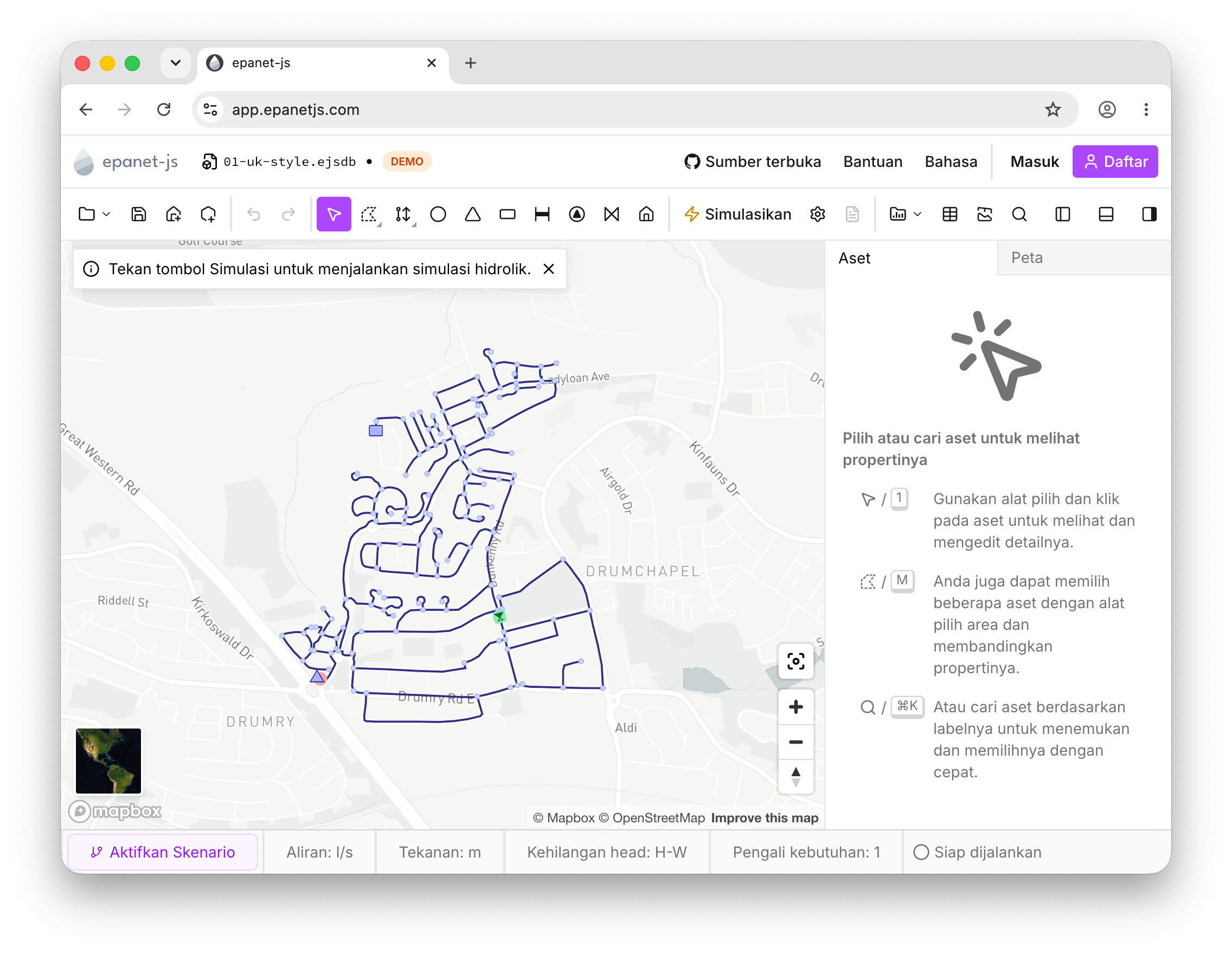
Alongside those, we’ve shipped time-series custom graphs, full data export (assets and simulation results to GeoJSON, CSV, Shapefile, and Excel), a new native project file (.ejsdb), pipe material and installation-year attributes, zone import, and experimental Indonesian language support.
And we’re turning one. Join us at the end of the month for a live Office Hours session to celebrate epanet-js’s first anniversary — details just below.
Office hours: our first anniversary
When we launched epanet-js, our mission was simple: make hydraulic modelling free, open-source, and accessible to anyone, anywhere, right from a web browser. One year later, we’re incredibly proud of how this community has grown and how you’ve used the tool to break free from the complexity of traditional modelling packages.
To celebrate, we’re hosting a live Office Hours session on Tue, Jun 30, 2026, 10:00 AM EST. We’ll open with a quick tour of the newest features — including HGL profiles and data tables — and share where we’re taking epanet-js next. Then we’ll do what these sessions do best and hand the floor to you: the most valuable, high-energy moments always come from your questions, so we’re keeping the bulk of the hour open for live Q&A.
Whether you’re curious about a specific feature, brainstorming a new workflow, or want to talk about the future of water modelling, bring your questions, ideas, and feedback to help shape the next chapter of the tool.
- When: Tuesday, Jun 30, 2026, 10:00 AM EST
- Your host: Luke Butler, co-founder of epanet-js.
Have a question already? Submit it when you register and we’ll line it up so we can hit the ground running. Can’t make it live? Register anyway and we’ll send you the full recording to watch on-demand.
Register now to save your spot
Priority access
You may notice a new prompt when you reach for certain features. To keep epanet-js sustainable, new premium features now debut to our paid plans and Founding Partners first, for their first 30 days. After that, they roll out to everyone.
When you open one of these features on the free plan, you’ll see a gentle nudge — Priority access — letting you know it’s available and making it easy to upgrade if you’d like it right away. Nothing is taken away: the free version keeps everything it has today, and every priority-access feature becomes free 30 days after launch.
This month, HGL profiles and time-series custom graphs are available through priority access.
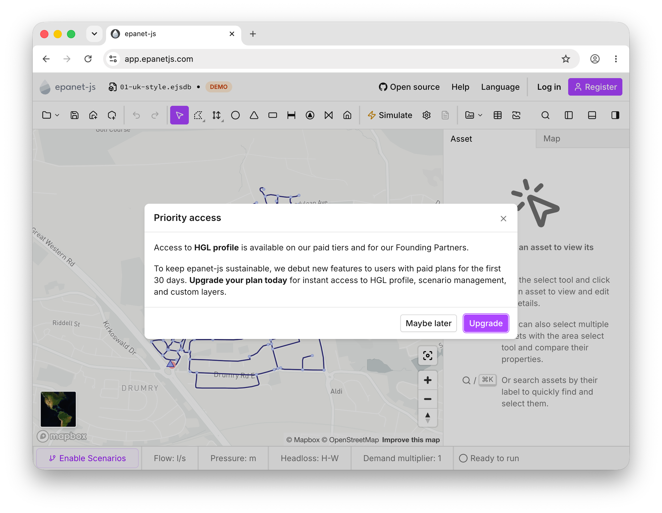
The priority access prompt, shown when you open a new feature on the free plan.
HGL profile
Priority accessThis is one of the two big ones this month. The HGL profile tool lets you visualise the hydraulic grade line and terrain along any path in your network, making it easy to spot pressure issues at a glance — and we’ve put a lot of work into making it both powerful and genuinely intuitive.
Pick the HGL profile from the toolbar, then choose a start and end point; epanet-js automatically traces the shortest path between them. If you need a specific route, keep clicking junctions to guide the path exactly where you want it, and hit escape when you’re done — the profile follows pipes, pumps, and valves anywhere along the way. Terrain is overlaid automatically from the map, so you can see how your network sits against the ground above it.
The chart is fully interactive and stays in sync with the map. As you move your cursor across the plot, a tracking cursor moves along the map at the same time, showing the exact pressure at each junction and interpolated values in between. You can zoom and pan the chart, and click any asset directly on the graph to open its properties.
A blue shaded band shows the full range of head along the route across the entire simulation — its absolute minimum and maximum extent. As you play back or step through the timeline, the current HGL line moves up and down within that band, making it easy to read how the system behaves and to spot critical high and low points along the route.
Asset data tables
Another long-requested feature, and the second big one this month. Asset data tables give you a spreadsheet-like view of all your network assets, making it easy to review, edit, and manage your model data in bulk. Every asset type is covered — junctions, pipes, pumps, valves, tanks, reservoirs, and customer points — and you can edit properties such as labels, elevations, and demands directly in the table. When a simulation is available, its results sit alongside your model properties.
A few things make the tables quick to work with:
- Sort by any column to find and compare assets at a glance.
- Copy and paste data straight in and out, with an option to include column headers.
- Delete assets directly from the table through the right-click menu.
- Bulk-edit demands across junctions and customer points in one go.
Time-series custom graphs
Priority accessTime-series custom graphs let you visualise how hydraulic values change over time for any combination of selected nodes and links, giving you a detailed view of your network’s behaviour across an extended period simulation. Pick the assets you’re interested in, choose a property — pressure, head, flow, velocity, headloss, status, or water quality — and the values are plotted together on a single chart, with nodes and links on separate Y-axes so the scales stay readable.
When you’re done, export the chart as a PNG or download the underlying data as CSV or XLSX. The graphs need an EPS (extended period) simulation to display data.
Export your data
Getting your data out of epanet-js is now much easier. Two new export tools cover both your model and your results.
Export asset data
Export asset data lets you download your network’s assets and their properties in the format you prefer — GeoJSON, CSV, Shapefile, or XLSX — ready to use in other tools. You can optionally include simulation results for the current timestep, and export either your whole network or just the assets you’ve selected.
Export simulation results
Export simulation results lets you download the full time-series output from an EPS simulation, giving you complete access to your hydraulic data outside the app. Export to CSV or XLSX, and choose exactly which properties to include: pressure, head, demand, flow, velocity, headloss, status, and water quality. As with asset data, you can export everything or just a selection.
Large exports show a warning with an estimated file size before you commit, and long-running exports can be cancelled at any point.
The epanet-js project file (.ejsdb)
Until now, epanet-js worked directly with standard .inp files. That’s still fully supported, but .inp was never designed to hold everything a modern model needs. This month we’re introducing a new native project file: .ejsdb.
The .ejsdb format stores everything a standard .inp can, plus the data that doesn’t fit in the EPANET format — customer points and zones among them.
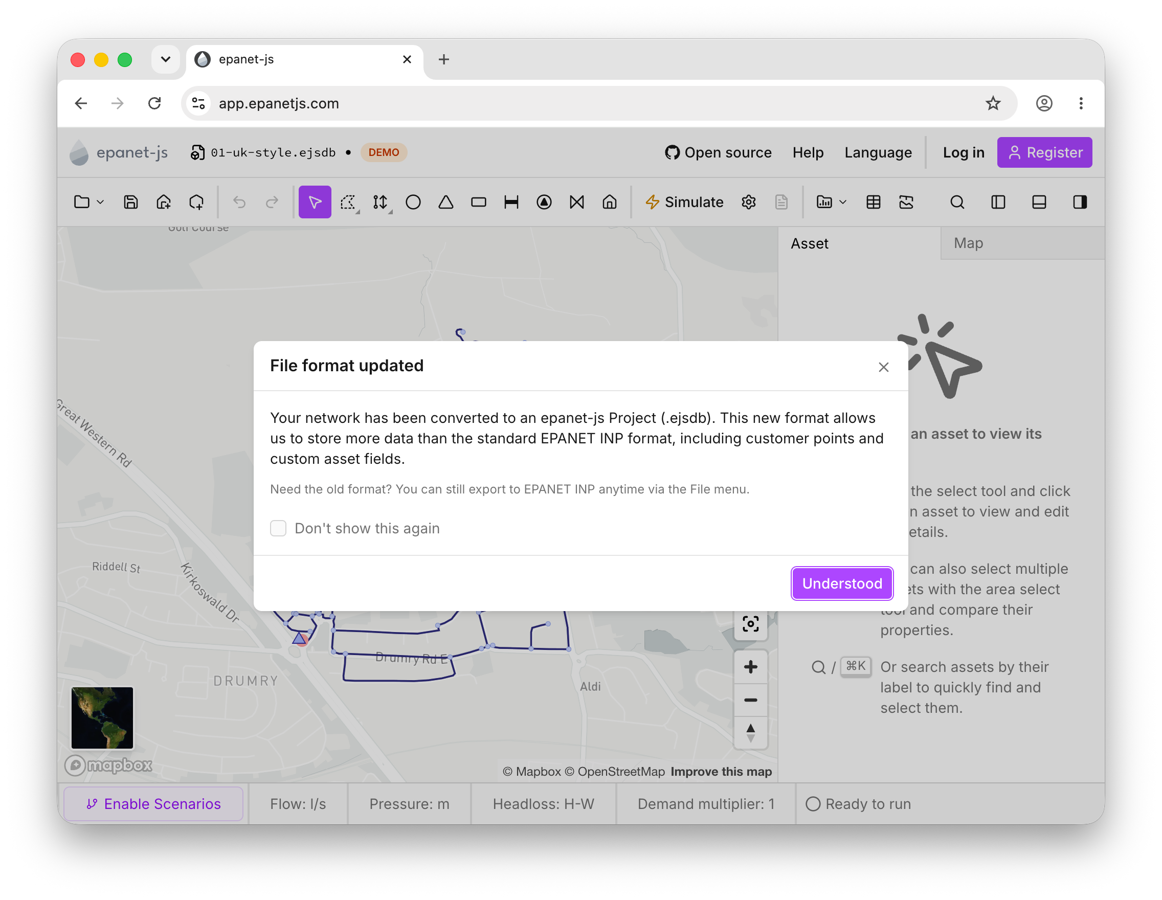
The new .ejsdb project file keeps customer points and zones that a standard .inp can’t store.
Model building
A couple of additions to help you enrich and organise your models.
Pipe material and installation year
Paid plansPipe material and installation year are optional attributes that let you enrich your pipe data with asset-management information, beyond what’s needed for hydraulic simulation. Set a material such as PVC or ductile iron on any pipe — picking an existing value or creating a new one — and record an installation year to track the age of your network. Both attributes are visible and editable in the asset panel, in the data tables, and through batch editing on multi-pipe selections.
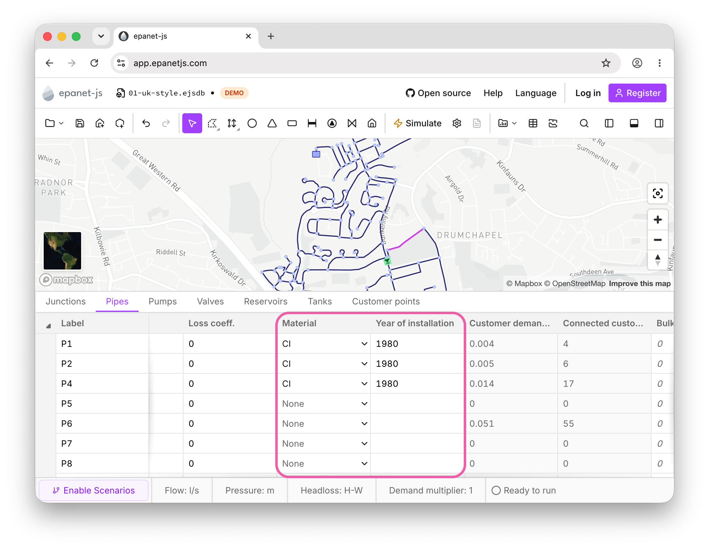
Set material and installation year on any pipe — in the panel, the data tables, or in bulk.
Zones
Paid plansYou can now import zone polygons from GIS data straight onto the map. Adjacent zones are automatically given distinct colors, so neighbouring areas never share a shade, and any polygons that share the same name are merged into a single zone. Zones are saved as part of the new .ejsdb project file.
This is just the foundation. Zones might look like a small feature today, but we have big plans for them. Soon you’ll be able to assign a selection of assets to a zone and make zones a much more dynamic part of the model — bulk-allocate customer points knowing every customer is correctly connected within its zone, and set default demands and patterns at the zone level for the assets inside to inherit, so you can test a different demand or pattern by changing it once and watching the whole zone update. You’ll also get zone-level statistics such as minimum and maximum pressure; because those are tied to the assets in the zone’s selection list, other assets crossing the area won’t throw off the numbers.
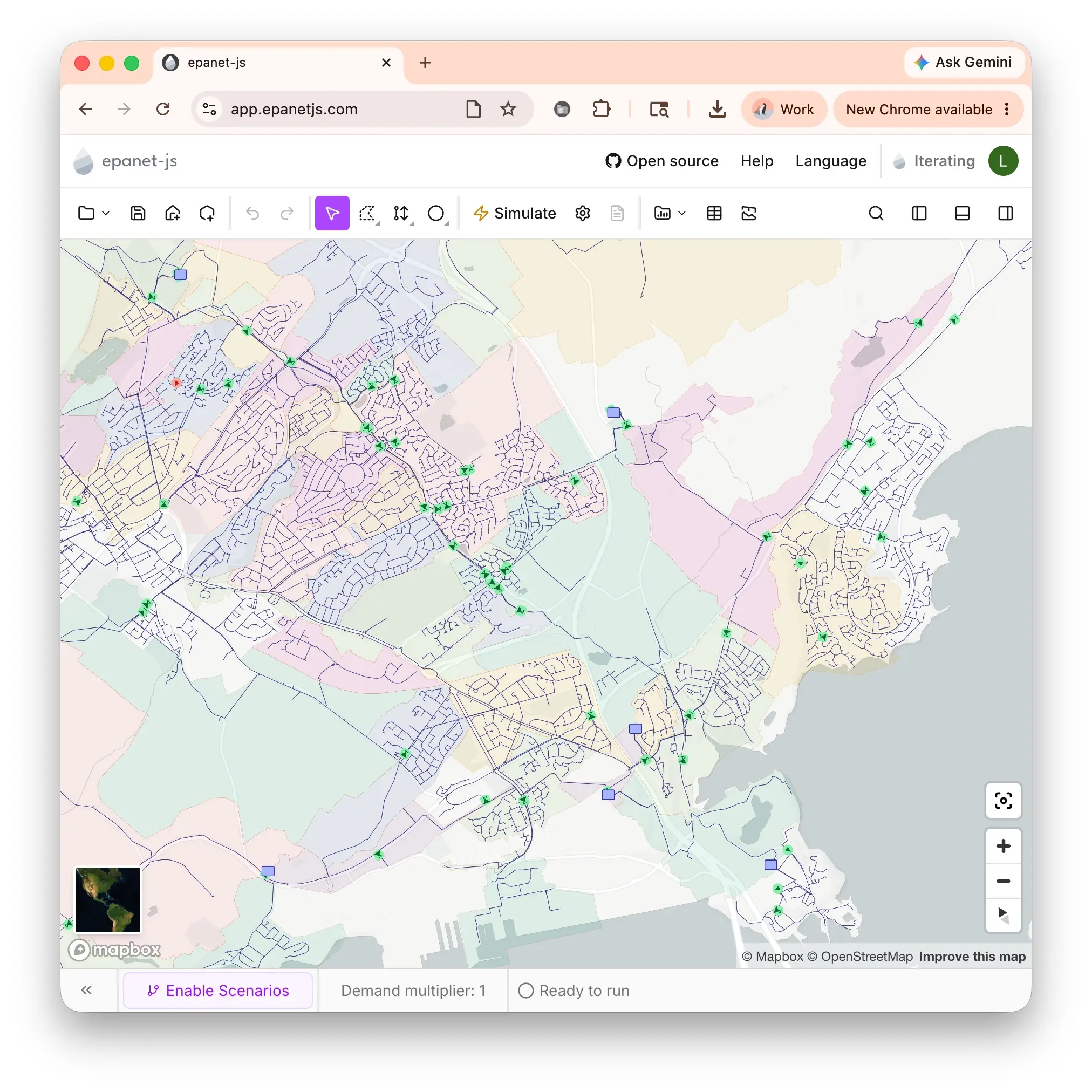
Import zone polygons from GIS data; adjacent zones are automatically given distinct colors.
Junction size and visibility
We heard from a lot of users that junctions could be hard to see in larger or rural networks, so we’ve added more control over how they appear on the map. In the node symbology under the Map tab, you can now adjust the size of junctions — setting a minimum size, a maximum size, and the zoom range over which they’re visible — so your network stays easy to read at any zoom level.
Indonesian language (experimental)
Indonesia is one of our fastest-growing user bases — more than 180 people used epanet-js there last month alone. After talking with Muhamad Safwan Irsyad and Zakky Rabbani at Mott MacDonald, who explained that while many modelers there are comfortable in English their clients would find the tool far more accessible in Bahasa Indonesia, we added a full Indonesian translation. With their help reviewing and correcting the text, it’s now available to every user.
It’s still an experimental language, but it’s a meaningful step toward making high-quality, open-source hydraulic modelling accessible to more teams around the world. As always, it’s a community effort, and it’s great to see engineers everywhere stepping up to help improve the tools for everyone.
Improvements
- Precision drawing at high zoom: When you’re zoomed in closely, the app now stores coordinates with higher precision, so assets land exactly where you place them, with no rounding drift.
- Min/Max pressure by node: Minimum and maximum pressure are now available as color-by options on the map. The values are computed across every timestep, so they reflect the whole simulation period rather than a single moment in time.
- Empty values in multi-asset stats: The multi-asset panel now includes “empty” values in its stats for optional attributes.
- Edit first demand from the data table: You can now set a junction’s first demand directly in the data tables.
- Sticky label column: The asset label column is now pinned to the left of the data tables. When scrolling horizontally through wide tables, the label stays fixed so you always know which asset each row belongs to.
- Default demand on import: Set a default demand value when importing customer points.
- Import customer points from Shapefiles: You can now import customer points from Shapefiles, in addition to GeoJSON.
Fixes
- Pump head values (rather than headloss) are now shown in the quick graph.
- The valve headloss curve warning no longer appears on descending values.
- Data table row order stays fixed while you edit content.
Community and growth
Presenting at VLCTechFest
Sandra and Sam took epanet-js to VLCTechFest, where they spoke about the challenges of building a hydraulic modelling application for the web. EPANET has over 30 years of history as a desktop tool, and we’ve turned it into an open-source, local-first web app where everything runs directly on the user’s machine. The talk dug into what that actually takes — running heavy calculations off the main thread, managing large volumes of data in the browser, recreating “native” workflows on the web, and choosing a file format that holds up — along with what’s still genuinely hard, and what it takes to build something that works completely offline.

What’s next
Our focus now turns to model building — making it faster and more reliable to put an accurate model together. Here’s what’s coming:
- Pipe definition library: Create and manage a library of standardised pipe definitions — common materials, internal and external diameters, and roughness values. When building a model or importing from GIS, apply them in a click to keep your pipe properties consistent and dramatically speed up the work.
- Material and year from GIS: Import pipe material and installation year straight from your GIS data, building on the new attributes we added this month.
- Smarter zones: Use zones to make sure customer points are only ever assigned to assets within their own boundary.
Support EPANET by using software that supports it back.
— Luke and Sam